How Does Transfer Learning Improve Face Recognition Accuracy?

When an ensemble of three fine-tuned face recognition models votes together, it reaches 69.75% Top-1 accuracy on a 2,000-face dataset, nearly double the 33.75% achieved by a single fine-tuned VGGFace model. This course project report walks through the full pipeline that got us there: face alignment with MTCNN, aggressive data augmentation, transfer learning from VGGFace and FaceNet, and a 3-model ensemble classifier. If you are trying to build a face recognition system without millions of labeled images, the transfer learning and augmentation techniques here show how to get meaningful results from a small dataset.

Key Takeaways

• Transfer learning from pre-trained models (VGGFace, FaceNet) enables face recognition on a small 2,000-face dataset without training from scratch.
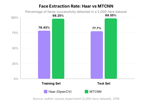
• MTCNN face alignment detects 98.25% of faces versus 78.45% for Haar cascades, and it rotates tilted faces to frontal (author experiment).
• A single fine-tuned VGGFace model overfits badly: 93.07% train accuracy but only 33.75% test accuracy (author experiment).
• An ensemble of three diverse models lifts Top-1 accuracy from 44.6% to 69.75% and Top-5 from 61.15% to 82.1% (author experiment).
• FaceNet's 128-dimensional Euclidean distance enables fast lazy learning: pre-compute face embeddings once, then compare in milliseconds.

What Is Transfer Learning for Face Recognition?

Transfer learning reuses a model trained on a large dataset as the starting point for a new task with less data. In face recognition, this matters because collecting and labeling millions of face images is expensive, yet the core features (edges, textures, facial geometry) learned on a big dataset transfer well to a new set of faces.

The research history of face recognition is long-standing. As early as 1888 and 1910, Galton published two articles in Nature on using faces for personal identification, analyzing humans' own ability to recognize faces. For most of the 20th century, automatic face recognition remained out of reach. Early work treated it as a pattern recognition problem using geometric feature-based methods, then appearance-based models like Eigenface, Fisherface, and elastic graph matching. By the late 1990s, researchers tackled real-world conditions with Linear Discriminant Analysis, kernel-based nonlinear methods, 3D face recognition, and local descriptors such as Gabor Face and LBP Face.

The turning point came in 2014. Deep learning combined with massive labeled face data became the mainstream approach. Facebook's DeepFace, published at CVPR 2014, trained on 4 million face images and approached human-level accuracy on the LFW benchmark (Taigman et al., DeepFace, 2014). Google's FaceNet, published at CVPR 2015, surpassed human-level accuracy using the Triplet Loss function (Schroff et al., FaceNet, 2015). These models proved that features learned on web-scale face data generalize, which is exactly what transfer learning exploits.

How Do FaceNet and VGGFace Work?

FaceNet and VGGFace are the two pre-trained architectures this project builds on. Both learn a compact embedding where similar faces cluster close together, but they differ in how they train and how you use the output.

FaceNet trains a deep convolutional network to map each face to a 128-dimensional vector, then optimizes the vectors so that same-person faces are close and different-person faces are far apart. It uses the Triplet Loss function: for each anchor face, it pulls the embedding toward a positive (same person) and pushes it away from a negative (different person). Google's original model trained on 200 million images of 8 million people and reached 99.63% accuracy on the LFW dataset (Schroff et al., FaceNet, 2015), effectively ending the eight-year LFW benchmark race.

Citation capsule: FaceNet maps each face to a 128-dimensional embedding and trains with triplet loss on 200 million images of 8 million people, reaching 99.63% accuracy on the LFW benchmark (Schroff et al., FaceNet, 2015). At the time, it was the highest reported result and marked the conclusion of the LFW performance competition.

VGGFace, from the Visual Geometry Group at Oxford, takes a different path. It uses VGGNet as the backbone and trains with standard softmax classification on the VGGFace dataset. After training, you remove the final classifier layer and use the penultimate score vector as the face feature, then compute Euclidean distance for verification. The authors reported 98.95% accuracy on LFW (Parkhi et al., VGGFace, 2015). The score vector can be refined further with triplet loss in Euclidean space.

For face detection and alignment, this project also uses MTCNN, a cascaded convolutional neural network published at ECCV 2016 (Zhang et al., MTCNN, 2016). MTCNN runs three networks in sequence: P-Net proposes candidate face windows, R-Net refines them by rejecting false positives through an extra fully connected layer, and O-Net adds finer-grained supervision and outputs five facial landmarks.

How Do You Align Faces Before Recognition?

Face alignment normalizes each detected face so that two images of the same person can be compared fairly. The main operations are cropping and rotation, which remove background noise and correct for head tilt. This project compares two alignment methods: Haar cascades via OpenCV and MTCNN.

Face Extraction Using OpenCV Haar Features

Haar features capture grayscale variations in an image. OpenCV ships with XML files pre-trained on facial features that you can load to detect faces (OpenCV haarcascades). This project uses five cascade files:

haarcascade_frontalface_default.xml
haarcascade_frontalface_alt.xml
haarcascade_frontalface_alt2.xml
haarcascade_frontalface_alt_tree.xml
haarcascade_profileface.xml

The first four detect frontal faces; the last one detects profile faces. Below is an example of the extraction results:

Original Image	Extracted Image

The actual extraction results on our dataset:

Training Set Count	Training Set Percentage	Test Set Count	Test Set Percentage
1,569	78.45%	1,554	77.7%

Face Extraction Using MTCNN

MTCNN is a 2016 ECCV paper that uses a cascaded CNN for facial landmark detection and alignment (Zhang et al., MTCNN, 2016). This project uses the MXNet implementation for face alignment. An example:

Original Image	Extracted Image

The actual extraction results:

Training Set Count	Training Set Percentage	Test Set Count	Test Set Percentage
1,965	98.25%	1,971	98.55%

MTCNN not only finds more faces than Haar cascades (98.25% vs 78.45% on the training set), it also rotates tilted faces to frontal. That rotation step is what makes the biggest difference for downstream face comparison.

How Does Data Augmentation Improve Generalization?

In deep learning, more training data usually means better generalization. Since this project works with a small face dataset, data augmentation artificially expands the set by applying random transformations to each image. Two libraries handle this: Keras' ImageDataGenerator and the imgaug package.

Data Augmentation Using ImageDataGenerator

ImageDataGenerator is a Keras API that applies on-the-fly transformations during training:

• Rotation/reflection: randomly rotate the image by a set angle and flip its orientation
• Flip: mirror the image horizontally or vertically
• Zoom: enlarge or shrink the image by a random ratio
• Shift: translate the image on the plane, horizontally or vertically
• Scale: resize the image or filter it to build a scale space, changing size or blurriness
• Contrast: change the saturation and brightness (S and V in HSV) while keeping hue fixed, applying an exponential factor between 0.25 and 4 to each pixel
• Noise: perturb each pixel's RGB values with salt-and-pepper or Gaussian noise

Four examples of generated augmentations:

Augmentation Example 1	Augmentation Example 2	Augmentation Example 3	Augmentation Example 4

Data Augmentation Using imgaug

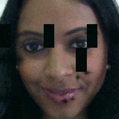
imgaug is a standalone Python library for image augmentation (imgaug). It supports image scaling, cropping or padding, horizontal and vertical flips, grayscale conversion, Gaussian perturbation, sharpening, embossing, and brightening or darkening.

Four more examples:

Augmentation Example 1	Augmentation Example 2	Augmentation Example 3	Augmentation Example 4

The pipeline generated 91,702 training images in total, an average of 44.85 augmented images per original training image.

Can Finetuning VGGFace Work on a Small Dataset?

Finetuning takes a model pre-trained on a large dataset and continues training it on your specific data. This experiment starts from the VGGFace RESNET50 model, keeps all weights before the fully connected layer, and retrains only the fully connected layer on the augmented training set.

On GitHub, rcmalli provides Keras implementations of VGGFace trained on the Oxford VGGFace dataset, with VGG16, RESNET50, and SENET50 backbones (rcmalli/keras-vggface). This project uses the RESNET50 variant. The training and validation accuracy curves are shown below:

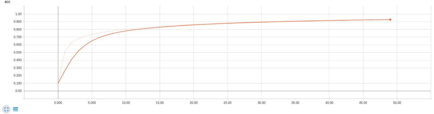
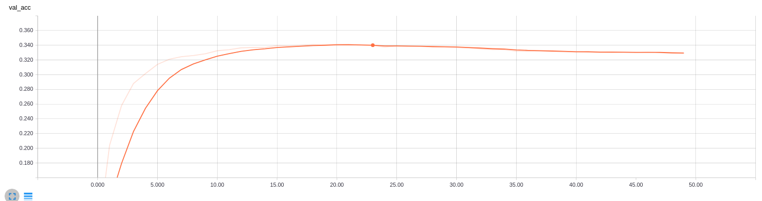
After 50 epochs, the training accuracy reached 0.9307 while the test accuracy peaked at only 0.3375. Top-1 accuracy was 0.3375 and Top-5 accuracy was 0.489. The large gap between train and test accuracy is a clear sign of overfitting: the model memorized the augmented training faces instead of learning features that generalize.

What Is Lazy Learning and How Does FaceNet Compare Faces?

Lazy learning skips explicit model training at prediction time. Instead, it computes the distance between each test sample and every training sample, then returns the closest match. FaceNet makes this practical because it compresses each face into a 128-dimensional vector, so comparing two faces is just a Euclidean distance calculation.

The FaceNet model used here is davidsandberg's implementation, trained on VGGFace2 with an Inception ResNet v1 architecture, which reports 0.9965 accuracy on LFW (davidsandberg/facenet). The process is straightforward:

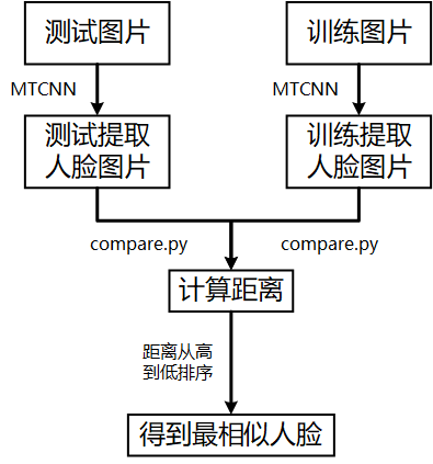
MTCNN first extracts the face region from the input image. Then a pre-computed compare script calculates the similarity between pairs of images. Because each test image must be compared against all 2,000 training images, pre-computing and caching the face embeddings to disk speeds things up dramatically.

An example of the raw face distances:

0          0       1.3858
0          1       1.3257
0          2       1.5103
0          3       1.1707
0          4       1.0327
0          5       1.4050
0          6       1.5472
0          7       1.3509
0          8       1.3133
0          9       1.4988

The first column is the test image index, the second is the training image index, and the third is the Euclidean distance between their embeddings.

After sorting all distances and taking the top 5 matches:

120:332,120,1534,405,356
121:121,193,1536,1252,1984
122:122,987,1165,780,1317
123:123,1077,1154,135,1222
124:550,600,124,1292,589
125:953,549,125,1981,1729
126:126,138,1820,1699,462
127:127,1003,1013,1441,325
128:201,817,1002,2,717

The number before the colon is the test image index; the numbers after are the indices of the 5 closest training faces.

Using the original pre-trained FaceNet model without finetuning, Top-1 accuracy was 0.446 and Top-5 accuracy was 0.6115.

How Do Ensemble Classifiers Boost Accuracy?

A single model has blind spots. An ensemble combines multiple diverse models so that one model's strength can cover another's weakness. This project builds three base classifiers that differ in their loss functions, training data, and image processing:

• Model 1: no finetuning, original images processed with MTCNN
• Model 2: softmax loss + center loss, 2,000 training images and 2,000 grayscale images, processed with both MTCNN and OpenCV
• Model 3: triplet loss, 2,000 training images and 8,000 augmented images, grayscale images processed with both MTCNN and OpenCV

The ensemble uses a KNN classifier (k=1, Euclidean distance) on each model's output and combines the three predictions.

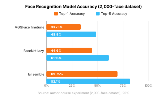
The ensemble lifted Top-1 accuracy from 44.6% (single best model) to 69.75%, and Top-5 accuracy from 61.15% to 82.1%. The diversity across loss functions, training sets, and image preprocessing is what drives the gain: each model makes different errors, so the majority vote cancels them out.

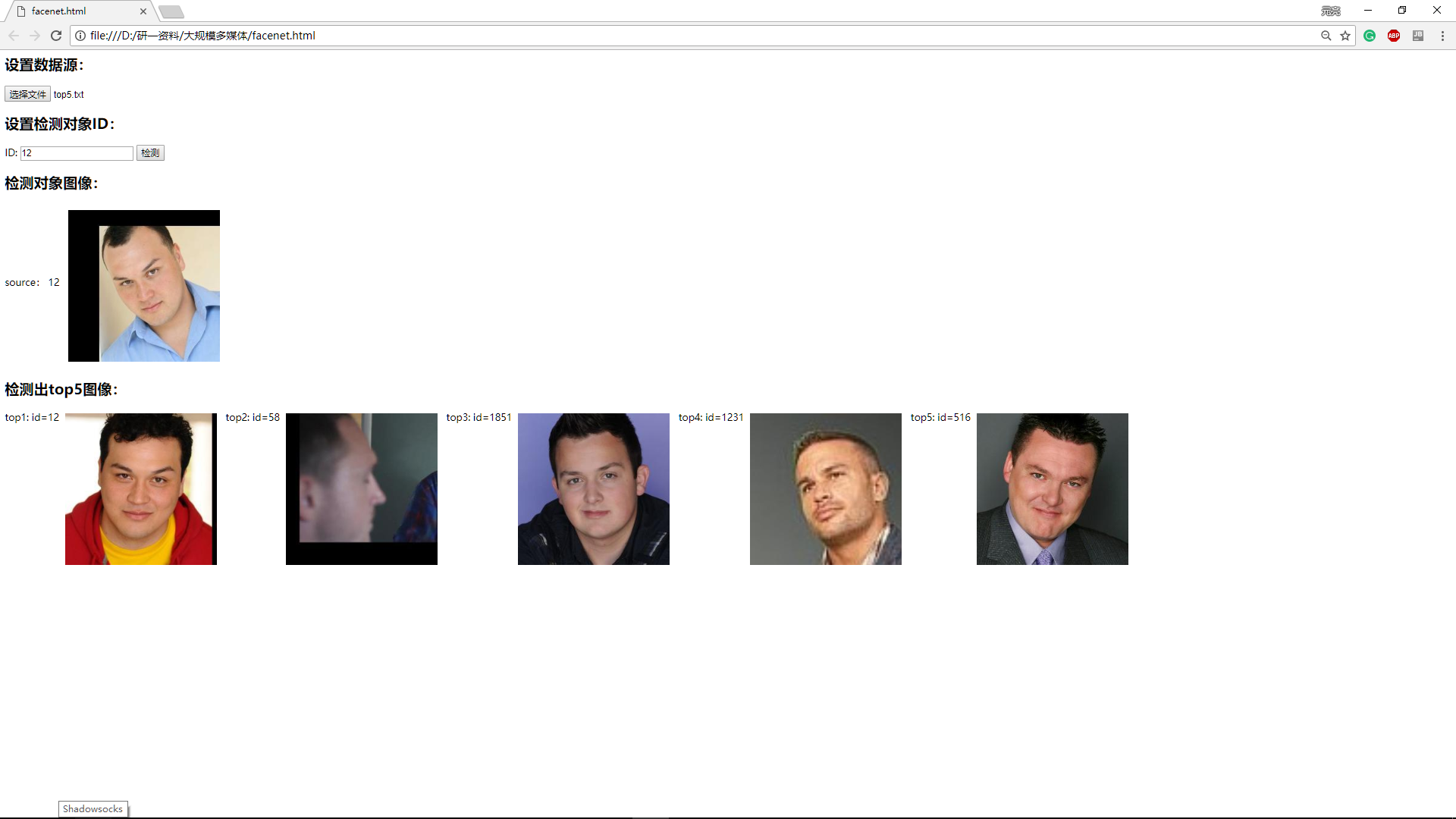
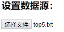
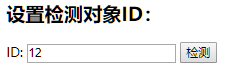
The interface lets you run the final model and query any test identity:

Run the final result data from the imported model	Input the ID of the object to be detected

The system returns the 5 closest matching faces:

Frequently Asked Questions

What dataset was used in this experiment? The dataset contains 2,000 face images collected for a university course project. After MTCNN extraction and augmentation, the training set grew to 91,702 images (44.85 augmented versions per original image).

Why use MTCNN instead of Haar cascades for face alignment? MTCNN detected 98.25% of faces in the training set versus 78.45% for Haar cascades. More importantly, MTCNN rotates tilted faces to frontal before comparison, which directly improves downstream recognition accuracy.

What is the triplet loss function FaceNet uses? Triplet loss takes an anchor face, a positive face (same person), and a negative face (different person), then trains the network so the anchor is closer to the positive than to the negative by a margin. FaceNet's 128-dimensional output makes this distance meaningful.

Why does the fine-tuned VGGFace model overfit so badly? Training accuracy reached 93.07% but test accuracy peaked at only 33.75%. The model memorized the augmented training variants rather than learning generalizable facial features. A larger dataset or stronger regularization would help.

Can this transfer learning approach scale to larger face datasets? Yes. the same pipeline (MTCNN alignment, augmentation, pre-trained base models, and ensembling) scales naturally. On larger datasets, finetuning the full network (not just the classifier) and using harder triplet mining would push accuracy higher.

Conclusion

This project applied transfer learning to face recognition on a 2,000-face dataset and reached 69.75% Top-1 and 82.1% Top-5 accuracy through a 3-model ensemble. The pipeline (MTCNN alignment, aggressive augmentation, VGGFace and FaceNet finetuning, and ensemble voting) shows that meaningful face recognition is possible without web-scale data.

Several directions could push the results further. First, ensembling dlib, Haar, and MTCNN for alignment would recover even more faces from difficult angles. Second, extracting individual facial features (eyes, nose, ears) and training separate classifiers on each, then combining them with majority voting, could reduce the frontal-to-profile matching errors we observed. Third, TP-GAN style models can synthesize frontal faces from profile views, which would address the single biggest source of misclassifications in our tests.

Sources

• Taigman et al., "DeepFace: Closing the Gap to Human-Level Performance in Face Verification," CVPR 2014, https://research.facebook.com/publications/deepface-closing-the-gap-to-human-level-performance-in-face-verification/
• Schroff et al., "FaceNet: A Unified Embedding for Face Recognition and Clustering," CVPR 2015, https://arxiv.org/abs/1503.03832
• Parkhi et al., "Deep Face Recognition," BMVC 2015, https://www.robots.ox.ac.uk/~vgg/publications/2015/Parkhi15/parkhi15.pdf
• Zhang et al., "Joint Face Detection and Alignment using Multi-task Cascaded Convolutional Networks," ECCV 2016, https://arxiv.org/abs/1604.02878
• OpenCV, "Haar Feature-based Cascade Classifier for Object Detection," https://github.com/opencv/opencv/tree/master/data/haarcascades
• aleju, "imgaug," image augmentation library, https://github.com/aleju/imgaug
• rcmalli, "keras-vggface," VGGFace models in Keras, https://github.com/rcmalli/keras-vggface
• davidsandberg, "facenet," FaceNet implementation in TensorFlow, https://github.com/davidsandberg/facenet