Can We Predict Whether You'll Replay a Song? Mining KKBOX's Music Data

KKBOX is a leading music streaming service in Asia with one of the world's most comprehensive collections of Asian pop music. The company released a dataset through Kaggle's music recommendation challenge — and we used it to answer a concrete question: can we predict whether a user will replay a particular song within a month? Using LightGBM with 10-fold cross-validation, we achieved a 0.792 average AUC. Along the way, we clustered listeners and songs with K-prototypes, visualized the results with t-SNE, and found that a song's singer, lyricist, and composer matter far more than user demographics for predicting repeat plays.
Introduction
The KKBOX music recommendation dataset contains four tables — members, songs, song extra info, and listening logs — that let us explore four connected data-mining problems. We analyzed feature correlations, clustered users by listening habits, clustered songs by metadata, and built a repeat-playment predictor. Each experiment used a different algorithm chosen for the data's shape: Pearson correlation for feature analysis, K-prototypes for mixed numeric-categorical clustering, t-SNE for high-dimensional visualization, and LightGBM for gradient-boosted prediction. This post walks through what we did, what worked, and what we'd do differently.
Key Takeaways
- A LightGBM model trained on KKBOX's Kaggle dataset achieved a 0.792 average AUC (10-fold cross-validation) predicting whether a user replays a song within a month.
- K-prototypes clustering (k = 20 for users over 100 iterations, k = 50 for songs over 200 iterations) produced coherent groups validated by t-SNE visualization.
- A song's singer, lyricist, and composer are the strongest predictors of repeat plays — user age and gender barely matter.
- Listening channel, page, and song source are highly correlated in practice, which makes sense: a search on the search page usually leads to an online playlist.
- For a related recommendation-system project, see How Can a Big Data Platform Match Over a Million Resumes to the Right IT Jobs?
How Do Features in the Listening Dataset Correlate?
The dataset's features aren't independent — channel, page, and source tend to move together. We started by quantifying those relationships.
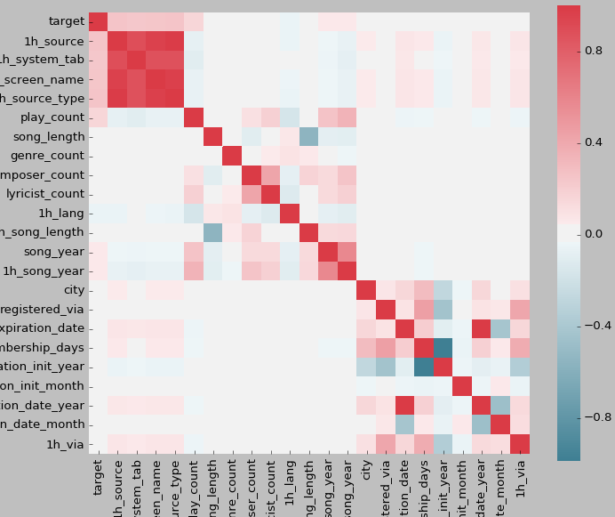
We selected train.csv as the data source and cleaned it: counting genres and songwriters, one-hot encoding categorical fields like language, system_tab, screen_name, source_type, and year, binarizing song length, and handling missing values and outliers. After processing, we had 23-dimensional features and computed pairwise Pearson correlations across all dimensions.
The result: 1h_source, 1h_system_tab, 1h_screen_name, and 1h_source_type show high correlation with each other, while other dimensions correlate weakly. These four fields describe repeat-play probability, the channel that triggered the repeat, the page it happened on, and the song's source — and the "1h" prefix means they're one-hot encoded. This makes practical sense. A user who replays a song through search usually does so on the search page, listening to an online playlist. The search channel, search page, and online playlist co-occur naturally, and since all three describe repeat-play behavior, each correlates strongly with the repeat-play rate.
How Can We Cluster Music Listeners Into Similar Groups?
Listeners who behave alike should cluster together — that's the foundation of segment-based recommendation. We tested whether K-prototypes could find those segments in mixed-type user data.
We processed members.csv and train.csv to extract registration year/month/day, membership duration, total songs played, total repeat-played songs, and repeat-play rate, encoding gender as male (0), missing (1), female (2). Because the dataset contains discrete attributes like user IDs alongside numeric ones, standard K-means wouldn't work — so we used K-prototypes, which Huang [1] designed specifically for mixed numeric-categorical data by combining K-means and K-modes with a weight parameter γ.
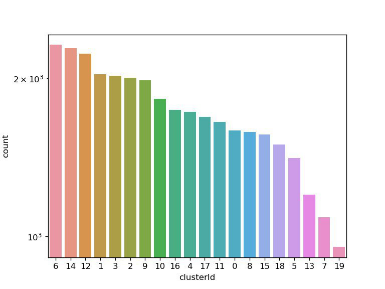
We ran K-prototypes with k = 20 for 100 iterations, then tabulated the cluster sizes. The largest cluster holds over 2,000 users; the smallest, a few hundred. The distribution is relatively even — no single cluster dominates. To check quality, we projected the high-dimensional results into 2D with t-SNE (t-Distributed Stochastic Neighbor Embedding) [3], an improvement over SNE [2] that preserves local structure by mapping points to probability distributions and matching them in low-dimensional space.
| Figure 2 — Records per user cluster | Figure 3 — t-SNE visualization of user clusters |
|---|---|
 |
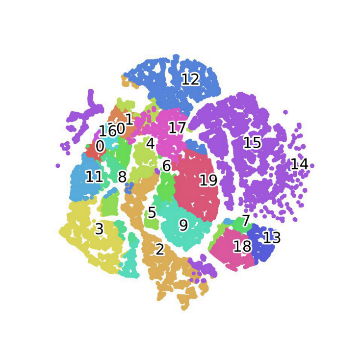 |
Figure 3 shows that points of the same category mostly aggregate into tight groups — users within the same cluster have high behavioral similarity. That's exactly what you want for segment-based recommendation: if you know a user's cluster, you can recommend what similar listeners enjoy.
How Do We Group Songs by Similarity?
The same clustering logic applies to songs. If we can group similar songs together, recommendation becomes a matter of suggesting tracks from the same cluster a user already likes.
We processed songs.csv and train.csv to extract release year, genre count, number of singers, lyricists, and composers, plus play count and repeat-play count per song. Missing release years were imputed with the mode. Again, because song IDs and singer names are discrete, we used K-prototypes — this time with k = 50 for 200 iterations.
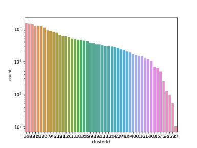
| Figure 4 — Records per song cluster | Figure 5 — t-SNE visualization of song clusters |
|---|---|
 |
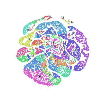 |
The largest song cluster holds over 100,000 tracks; the smallest, around 100. Figure 5 shows 50 color-coded classes, and again, same-category points mostly cluster together — songs in the same group share measurable similarity.
A concrete example makes this tangible. Two Jay Chou songs — "園遊會" (Garden Party) and "公公偏頭痛" (Grandpa's Migraine) — both co-written with lyricist Vincent Fang, landed in Cluster 6. Their styles are similar, and the algorithm grouped them together without knowing anything about genre labels. That's the clustering working as intended: you can recommend same-cluster songs to a user who listens to one of them.
| Clustering Result |
|---|
| 253492, 465, 周杰倫 (Jay Chou), 周杰倫, 方文山, 3.0, 園遊會, TWK970400709, 6 |
| 166661, 458, 周杰倫 (Jay Chou), 周杰倫, 方文山, 3.0, 公公偏頭痛, TWK971601115, 6 |
Can We Predict Whether a User Will Replay a Song?
This is the core recommendation problem: given a user and a song, will they listen to it again within a month? We treated it as a binary classification task and trained a LightGBM model.
LightGBM [4], proposed by Ke et al., is a distributed gradient-boosting framework that speeds up traditional GBDT by over 20× at nearly the same accuracy. It achieves this through histogram-based tree building, leaf-wise growth with depth limits, histogram difference acceleration, direct categorical feature support, and multi-threaded optimization — all of which matter when you're training on KKBOX's listening logs.
We used the 23-dimensional features from the correlation analysis and trained with 10-fold cross-validation: split the training set into 10 subsets, use 9 for training and 1 for validation each round, compute AUC per round, and average the 10 results.
| Experiment Number | AUC |
|---|---|
| 1 | 0.802 |
| 2 | 0.801 |
| 3 | 0.802 |
| 4 | 0.801 |
| 5 | 0.802 |
| 6 | 0.800 |
| 7 | 0.788 |
| 8 | 0.775 |
| 9 | 0.775 |
| 10 | 0.771 |
The average AUC is 0.792. AUC ranges from 0 to 1 and represents the area under the ROC curve — the higher, the better. To understand why the model works, we computed feature importance using the average-accuracy-reduction method: randomly permute a feature's values and measure the accuracy drop on out-of-bag data. A big drop means the feature matters.
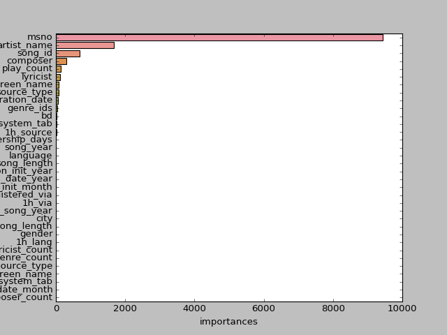
Two conclusions stand out:
- For a given song, whether it gets replayed depends mostly on its singer, lyricist, and composer — these are the key factors. Other song features barely move the needle.
- For a given user, repeat-play behavior has almost no relationship to basic demographics like age and gender. The strongest predictor is the user ID itself, which means individual listening habits vary enormously — almost like a random process. The practical takeaway: analyze what a user does, not who they are.
What Are the Limitations and Next Steps?
The results are promising but not ideal — that average AUC of 0.792 leaves room for improvement. We identified four concrete reasons and what we'd change:
- Missing-value handling was crude. Simple imputation (like the mode for song years) throws away information. A more careful approach — flagging missingness as a feature, or using model-based imputation — could help.
- We only tested a few k values. User clustering used k = 20; song clustering used k = 50. We didn't sweep systematically. The elbow method or silhouette score would find better cluster counts.
- Discrete variables in clustering were under-quantified. K-prototypes handles mixed types, but the categorical encoding could be richer — embeddings or target encoding might capture more signal.
- Clustering and prediction weren't integrated. The clusters we found were analyzed separately from the LightGBM model. Feeding cluster membership as a feature into the predictor could boost performance.
This was a classroom project, and its real value was turning data-mining theory into working code on a real dataset. The methods — correlation analysis, K-prototypes, t-SNE, LightGBM — are all standard tools, and seeing them connect raw logs to a measurable AUC result is what made the concepts click.
Frequently Asked Questions
What is the KKBOX dataset on Kaggle? It's the dataset from KKBOX's Music Recommendation Challenge, containing user listening logs, member profiles, song metadata, and extra song info. The goal is to predict whether a user will replay a song within a month based on their listening history and track features.
Why use K-prototypes instead of K-means for this data? K-prototypes, introduced by Huang [1], handles datasets with both numeric and categorical attributes — like our user and song tables, which mix play counts (numeric) with user IDs and singer names (categorical). K-means only works on numeric data, so it can't natively handle the categorical half.
What does an AUC of 0.792 mean in practice? AUC measures how well the model ranks positive cases (will replay) above negative ones (won't replay). At 0.792, there's a 79.2% chance the model ranks a random replayer higher than a random non-replayer. It's solid but not production-grade — most deployed recommenders target 0.85+.
How was t-SNE used to validate clustering results? t-SNE [3] projects high-dimensional cluster assignments into 2D while preserving local structure. When same-colored points (same cluster) appear grouped in the t-SNE plot, it confirms the clusters have meaningful internal cohesion — which we observed for both user and song clusters.
Sources
- KKBOX, KKBOX Music Recommendation Challenge (Kaggle), https://www.kaggle.com/competitions/kkbox-music-recommendation-challenge
- Huang ZX, Michael KN, "A fuzzy k-modes algorithm for clustering categorical data," IEEE Trans. on Fuzzy System, 1999, 7(4): 446–452
- Hinton GE, Roweis ST, "Stochastic neighbor embedding," Advances in Neural Information Processing Systems, 2002
- Van der Maaten L, Hinton G, "Visualizing Data using t-SNE," Journal of Machine Learning Research, 2008, 9: 2579–2605
- Ke G, Meng Q, Wang T, Chen W, Ma W, Liu TY, "A Highly Efficient Gradient Boosting Decision Tree," Advances in Neural Information Processing Systems, 2017, 3148–3156