Only Compile the Path You're Actually Running: The 'Precision Strike' Philosophy of Tracing JIT
V8's TurboFan compiles entire functions. Java's C2 compiler methods end-to-end. JavaScriptCore's DFG takes whole basic blocks and transforms them. These are method JITs — they see the full control-flow graph of a function and optimize all of it.
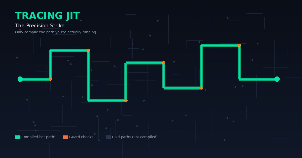
LuaJIT does something fundamentally different. It doesn't compile functions. It compiles paths — a single linear sequence of instructions that the program actually executed. If a loop runs 100 times, LuaJIT doesn't compile the loop body once; it records the exact path taken through those 100 iterations and compiles that.
This is the "precision strike" philosophy: instead of carpet-bombing the entire function with optimization, the tracing JIT fires a sniper bullet at exactly the code that matters. The result, for the right workloads, is faster warm-up, tighter code, and better performance on the hot paths that actually determine runtime.
In this article, you'll learn exactly how tracing JIT works — from hot path detection through recording, compilation, execution, and deoptimization. We'll trace the full pipeline and see why this approach is so effective for dynamic languages like Lua.
Key Takeaways
- Tracing JIT records a single hot path (linear trace), not a whole function — this is the fundamental design difference from method JIT.
- Type specialization happens naturally: the trace records actual types observed at runtime, and guards verify them on every execution.
- The compiled machine code lives in an
mmap'd memory buffer, flipped to executable viamprotect(), and called as a function pointer.- Deoptimization via snapshots makes aggressive speculation safe — guard failure reconstructs interpreter state and resumes.
- Side traces build trace trees that cover multiple paths through the same code, each compiled and linked together.
The Two Philosophies — Method JIT vs Tracing JIT
Every JIT compiler faces the same question: what do I compile? The answer defines the two schools of JIT design.
Method JIT (V8 TurboFan, Java C2, JavaScriptCore DFG/FTL, .NET RyuJIT) answers: "Compile the entire function." The compiler takes the function's bytecode, builds a control-flow graph (CFG) covering all basic blocks and branches, applies optimizations to the whole graph, and emits machine code for the entire function. Every path through the function gets compiled code.
Tracing JIT (LuaJIT, TraceMonkey, PyPy, Dynamo) answers: "Compile the path that just ran." The compiler waits until a loop or function entry becomes hot, then records the exact sequence of instructions executed — including which branches were taken, which types were observed, which functions were called. It compiles only that linear sequence.
 Method JIT (carpet bomb):              Tracing JIT (precision strike):

 ┌─────────────────────┐                ┌─────────────────────┐
 │  ┌───┐   ┌───┐      │                │  ┌───┐   ┌───┐      │
 │  │ A ├──▶│ B │      │                │  │ A ├──▶│ B │      │
 │  └─┬─┘   └─┬─┘      │                │  └─┬─┘   └─┬─┘      │
 │    ▼       ▼        │                │    ▼       ▼        │
 │  ┌───┐   ┌───┐      │                │  ┌───┐   ┌───┐      │
 │  │ C │   │ D │      │                │  │ C │   │ D │      │
 │  └─┬─┘   └─┬─┘      │                │  └─┬─┘   └─┬─┘      │
 │    ▼       ▼        │                │    ▼       ▼        │
 │  ┌───┐   ┌───┐      │                │  ┌───┐   ┌───┐      │
 │  │ E │   │ F │      │                │  │ E │   │ F │      │
 │  └───┘   └───┘      │                │  └───┘   └───┘      │
 │                     │                │                     │
 │  ALL blocks compiled │                │  Only A→B→D→F      │
 │  (entire CFG)       │                │  compiled (one path) │
 └─────────────────────┘                └─────────────────────┘
The tradeoff is coverage vs precision:
| Aspect | Method JIT | Tracing JIT |
|---|---|---|
| Compilation unit | Entire function | Single hot path |
| Optimization scope | Full control-flow graph | Linear trace |
| Warm-up speed | Slower (compiles everything) | Faster (compiles only hot code) |
| Peak performance | Higher (whole-function opts) | Lower per-trace, but traces are tight |
| Type specialization | Speculative, deopt on mismatch | Observed types, guards verify |
| Best for | Static languages, complex methods | Dynamic languages, tight loops |
| Memory usage | Higher (all code compiled) | Lower (only hot paths) |
Historically, tracing JIT was pioneered by Dynamo (2000), a transparent dynamic optimization system that recorded hot paths in native code. Mozilla's TraceMonkey (2009) brought it to JavaScript, achieving 2-20x speedups on some benchmarks before being replaced by method JITs. LuaJIT 2 (2010+) refined the approach with SSA IR, snapshot-based deoptimization, and trace trees — and remains the gold standard for tracing JIT performance.
How LuaJIT Detects Hot Paths
Tracing JIT starts with a simple question: which code is hot enough to compile? LuaJIT answers this with hot counters — execution counters embedded in the interpreter loop that decrement on every pass through a loop header or function entry.
The Hot Counter Mechanism
Every loop opcode (FORL, ITERL, LOOP) and function entry opcode (FUNCF, FUNCV) in the interpreter has an associated hot counter. The default threshold is 56 iterations — tunable via jit.opt.start('hotloop').
The mechanism lives in the DynASM-generated interpreter (src/vm_x64.dasc):
|->forl:                    ; Numeric FOR loop header
|  sub [hotcount], 1        ; decrement hot counter
|  jg >1                   ; if counter > 0, skip JIT check
|  call lj_trace_hot       ; counter hit zero — trigger JIT
|  jmp >2                  ; continue to loop body
|1:                        ; not yet hot — run interpreter
|  ...                     ; actual FOR loop logic
|2:                        ; fall-through after JIT check
When the counter reaches zero, lj_trace_hot() fires. This function transitions the JIT state machine from IDLE to START, allocates a new trace number, and begins recording.
The Trace State Machine
 ┌────────┐    hot counter=0    ┌─────────┐    recording    ┌──────────┐
 │  IDLE  │────────────────────▶│  START  │───────────────▶│ RECORD   │
 │        │                     │         │                │          │
 └────────┘                     └─────────┘                └────┬─────┘
      ▲                                                        │
      │                                                        │ trace ends
      │                                                        ▼
      │  trace done                                      ┌──────────┐
      │◀─────────────────────────────────────────────────│   END    │
      │                                                 └────┬─────┘
      │                                                      │ optimize
      │                                                      ▼
      │                                                 ┌──────────┐
      └─────────────────────────────────────────────────│   ASM    │
                                                        │ (compile)│
                                                        └──────────┘
The states:
- IDLE: Interpreter runs normally, hot counters decrement.
- START:
lj_trace_hot()fires, allocates trace, sets up recorder. - RECORD:
lj_record_ins()runs, translating bytecode to SSA IR. - END: Recording stops, trace is linked, optimizations run.
- ASM: The assembler emits machine code into an mmap'd buffer.
I-Prefixed Opcodes: The Bridge
LuaJIT's interpreter has two variants of loop and function opcodes: the normal versions (FORL, FUNCF) and I-prefixed versions (IFORL, IFUNCF). The I variants are patched in by the JIT once a trace is compiled — they coordinate with the recorder instead of running the full interpreter logic.
This is the bridge between interpreter and JIT: the same bytecode, but different opcode implementations depending on whether a trace exists.
Recording a Trace — Bytecode to SSA IR
Once recording starts, every bytecode instruction passes through lj_record_ins() — a 2,982-line master dispatch that translates bytecode operations into SSA (Static Single Assignment) intermediate representation.
The Recording Loop
// Simplified view of lj_record_ins()
void lj_record_ins(jit_State *J) {
  BCIns *pc = J->pc;           // current bytecode position
  BCOp op = bc_op(*pc);        // current opcode

  switch (op) {
    case BC_KSHORT: record_kshort(J, pc); break;
    case BC_ISNUM:  record_isnum(J, pc); break;   // type guard
    case BC_TGETV:  record_tgetv(J, pc); break;   // table get
    case BC_ADDVV:  record_addvv(J, pc); break;   // addition
    case BC_FORL:   record_forl(J, pc); break;    // loop
    // ... ~90 opcodes total
  }
}
Each record_* function emits one or more IR instructions via the emitir() macro:
#define emitir(ot, a, b) (lj_ir_set(J, (ot), (a), (b)), lj_opt_fold(J))This does two things: emit the IR instruction, then immediately run the FOLD engine on it for constant folding and simplification.
Type Specialization via Guards
The key to tracing JIT's performance is type specialization. In a dynamic language like Lua, a variable can hold a number, string, table, or function. A method JIT must generate code that handles all possibilities (or speculate and deopt). A tracing JIT records the actual type observed and emits a guard — a runtime check that verifies the assumption.
-- Lua source
local x = 0
for i = 1, 100 do
  x = x + i    -- x and i are both numbers here
end
The recorded IR for x = x + i:
 ─┬──────────────────────────────────────────────────────────────
 │  [1] ISEQ i, ┬──┬        ; guard: i is a number
 │              │  │
 │ [2] FLOAD x, ┼──┼──┬     ; load x from stack slot
 │              │  │  │
 │ [3] ADD   [2], ┼──┼──┬   ; x + i (both known to be numbers)
 │                │  │  │
 │ [4] FSTORE x, ─┴──┴──┴   ; store result back to x
 ─┴──────────────────────────────────────────────────────────────
The ISEQ instruction is a guard — it checks that i is indeed a number. If the check fails, the trace exits and deoptimizes. If it passes, the ADD instruction can use a single addsd (scalar FP add) instruction instead of a full polymorphic add.
On-the-Fly Optimizations During Recording
The recorder doesn't just translate — it optimizes as it goes. Every emitted instruction passes through the FOLD engine, which applies:
- Constant folding:
ADD(KNUM 3, KNUM 4)→KNUM 7(computed at record time) - Algebraic simplification:
ADD(x, 0)→x;MUL(x, 1)→x - Load forwarding (FWD): If a value was just stored and then loaded, skip the memory access
- Dead-store elimination (DSE): If a store is never read, remove it
- Narrowing (NARROW): If a double is guaranteed to be an integer, narrow to int32
These optimizations happen during recording, not after. This is unusual — most compilers separate recording/translation from optimization. But for a tracing JIT, the recording phase has perfect type information (from the guards), so optimizing immediately produces the tightest possible IR.
 Bytecode          Recording              On-the-fly opts           Final IR
 ───────          ──────────              ──────────────           ────────
 FORI  ──────▶  guard(i:int)  ──────▶  (fold constants)  ──────▶  guard(i:int)
 TGETV ──────▶  tgetv(tab,key) ──────▶  (fwd load)      ──────▶  tgetv → known offset
 ADDVV ──────▶  add(x,y)     ──────▶  (narrow to int)  ──────▶  add_i32(x,y)
 FORL  ──────▶  loop_exit?   ──────▶  (dse dead store) ──────▶  loop_link
Trace Linking and Side Traces — Building Trace Trees
A trace doesn't exist in isolation. When recording stops, LuaJIT determines what happens next — and this decision shapes the trace's relationship to other traces.
Trace End Conditions
Recording stops when:
- Loop back-edge: The trace reaches the loop header it started from →
LJ_TRLINK_LOOP(the trace loops to itself) - Guard failure: A guard fails during recording →
LJ_TRLINK_INTERP(exit to interpreter) - Function return: The trace reaches a return →
LJ_TRLINK_RETURN - Tail call: The trace reaches a tail call →
LJ_TRLINK_TAILREC - Call: The trace reaches a function call →
LJ_TRLINK_STITCH(trace stitching)
The most common case is the loop back-edge: the trace records one full iteration of the loop, then links back to its own start. Subsequent iterations run the compiled trace instead of the interpreter.
Side Traces: Covering Multiple Paths
A single trace covers one path through the loop. But real code has branches — what happens when the trace's guard fails at runtime? Instead of immediately falling back to the interpreter, LuaJIT can start a side trace that records the alternative path.
                    ┌─────────────────────┐
                    │   Parent Trace      │
                    │   (main loop path)  │
                    │                     │
                    │  guard(x > 0) ──────┼────┐ guard fails
                    │  ...                │    │ (x <= 0)
                    │  loop back ─────────┼─┐  │
                    └─────────────────────┘ │  │
                             ▲              │  │
                             │              │  ▼
                             │     ┌─────────────────────┐
                             │     │   Side Trace 1      │
                             │     │   (x <= 0 path)     │
                             │     │                     │
                             │     │  handle_negative()  │
                             │     │  exit to interp     │
                             │     └─────────────────────┘
                             │
                             │     ┌─────────────────────┐
                             │     │   Side Trace 2      │
                             │     │   (type mismatch)   │
                             │     │                     │
                             │     │  handle_string()    │
                             │     │  exit to interp     │
                             │     └─────────────────────┘
                             │
                    (loop back to parent)
When a guard fails enough times (default 10 failures, tunable via jit.opt.start('hotexit')), trace_hotside() starts a new recording from the interpreter state at that exit point. The new side trace is compiled and linked to the parent: lj_asm_patchexit() patches the parent trace's exit stub to jump directly to the side trace instead of returning to the interpreter.
The result is a trace tree — a tree of compiled traces covering multiple paths through the same loop. The root trace handles the common case; side traces handle the less common alternatives.
Trace Stitching
A special link type for call traces: when trace A calls a function that becomes hot and compiles to trace B, trace B is "stitched" — A's exit is patched to jump directly to B, avoiding the interpreter round-trip. The link field of A is set to B's trace number.
Trace Explosion and Blacklisting
The downside of trace trees: if a loop has many branches, each branch point can spawn side traces, and each side trace can spawn its own side traces. This trace explosion can consume significant memory.
LuaJIT mitigates this with blacklisting: if a particular bytecode location causes repeated deoptimization (more than a threshold number of times), LuaJIT stops tracing it. The location is marked as "not traceable" and the interpreter handles it forever. This prevents pathological cases where the JIT wastes time compiling traces that immediately deoptimize.
Snapshot-Based Deoptimization — The Safety Net
Tracing JIT's aggressive optimization relies on speculation: the trace assumes types, branch directions, and call targets based on what was observed during recording. When those assumptions hold, the trace runs at full speed. When they don't, the trace must deoptimize — exit the compiled code and resume in the interpreter.
Guards as Speculative Assertions
Every guard in the trace is a speculative assertion. The guard checks a condition (type, bounds, truthiness) and either continues or exits:
; Compiled trace code (x86-64)
movsd xmm0, [rbx+8]      ; load x
ucomisd xmm0, xmm0        ; check for NaN (is it a valid double?)
jp .exit_guard_3          ; if NaN, jump to exit stub
; ... continue trace ...
The jp .exit_guard_3 is the guard's exit path. If the condition fails, execution jumps to an exit stub — a small piece of code that saves the current state and calls the exit handler.
The Exit Handler and State Reconstruction
When a guard fails:
 ┌──────────┐    guard fails     ┌──────────────┐    fill state     ┌──────────────┐
 │  Trace   │──────────────────▶│  Exit Stub   │────────────────▶│ Exit Handler │
 │  (native)│                    │  (per-guard) │                  │ (lj_vm_exit_ │
 └──────────┘                    └──────────────┘                  │  handler)    │
                                                                   └──────┬───────┘
                                                                          │
                                                                          ▼
                                                                   ┌──────────────┐
                                                                   │ lj_snap_     │
                                                                   │ restore()    │
                                                                   │ reconstruct  │
                                                                   │ interp state │
                                                                   └──────┬───────┘
                                                                          │
                                                                          ▼
                                                                   ┌──────────────┐
                                                                   │ Interpreter  │
                                                                   │ resumes at   │
                                                                   │ restored PC  │
                                                                   └──────────────┘
- Exit stub saves all register and spill slot values to an
ExitStatestructure lj_vm_exit_handler(written in assembly) receives the exit number and register statelj_trace_exit()→trace_exit_cp()looks up the snapshot for this exitlj_snap_restore()reconstructs the interpreter state from the snapshot
Snapshot Structure
A snapshot lives at each guard point in the trace. It records:
- Which stack slots hold which IR references
- The call frame chain (PC + frame links for each active function)
- The machine code offset (so the exit handler knows which guard failed)
typedef struct SnapShot {
  uint32_t mapofs;    // Offset into snapshot map
  IRRef1 ref;         // First IR ref for this snapshot
  uint16_t mcofs;     // Offset into machine code
  uint8_t nslots;     // Number of valid slots
  uint8_t topslot;    // Maximum frame extent
  uint8_t nent;       // Number of compressed entries
  uint8_t count;      // Count of taken exits
} SnapShot;

typedef uint32_t SnapEntry;  // packed: slot(8) | flags(8) | ref(16)
Each SnapEntry encodes (slot << 24) + flags + ref where flags indicate whether the slot is a frame pointer, continuation, or needs no restoration.
Why This Matters
Snapshot-based deoptimization is what makes tracing JIT's aggressive optimization safe. The trace can assume types are constant, branches always go one direction, and call targets never change — because if any assumption fails, the snapshot provides a precise reconstruction of the interpreter state at that exact point.
This is fundamentally different from method JIT's deoptimization (on-stack replacement, or OSR), which must reconstruct state from a full CFG. Tracing JIT's snapshots are simpler because the trace is linear — there's only one possible state at each point.
How the JIT Actually Executes Machine Code
This is the mechanism that makes everything real: how does the compiled trace actually run? The answer involves the operating system's memory management — mmap and mprotect.
The MCode Allocation Pipeline
LuaJIT's JIT allocator (lj_mcode.c) manages regions of memory called MCode areas (default 64KB each, up to 2MB total). The pipeline:
 Step 1: mmap(RW)              Step 2: Assemble             Step 3: mprotect(RX)
┌──────────────────┐      ┌──────────────────┐      ┌──────────────────┐
│                  │      │  lj_asm.c writes │      │                  │
│  RW pages        │─────▶│  x86-64 bytes    │─────▶│  RX pages        │
│  (read-write)    │      │  into buffer     │      │  (read-execute)  │
│                  │      │                  │      │                  │
└──────────────────┘      └──────────────────┘      └──────────────────┘
        │                                                   │
        │                                                   ▼
        │                                          Step 4: Call
        │                                          ┌──────────────────┐
        │                                          │  Cast to fn ptr  │
        └─────────────────────────────────────────▶│  fn(T)           │
                                                   └──────────────────┘
Step 1 — Allocate RW memory:
// From lj_mcode.c — simplified
void *mcode_allocarea(jit_State *J, MSize sz) {
  void *p = mmap(NULL, sz, PROT_READ | PROT_WRITE,
                 MAP_PRIVATE | MAP_ANONYMOUS, -1, 0);
  // p is now a RW memory region — we can write to it, but not execute
  return p;
}
mmap with PROT_READ | PROT_WRITE allocates memory pages that can be written to but not executed. This is the W^X (Write XOR Execute) security principle: memory is never simultaneously writable and executable.
Step 2 — Write machine code:
// From lj_asm.c — the assembler writes bytes into the MCode buffer
void lj_asm_trace(jit_State *J, GCtrace *T) {
  MCode *mcarea = lj_mcode_reserve(J, &lim);  // get RW buffer
  // ... emit instructions byte by byte ...
  emit_loadi(RID_RET, 42);   // writes: 48 c7 c0 2a 00 00 00
  emit_jcc(CC_NE, exit_label); // writes: 75 XX (relative offset)
  // ...
  lj_mcode_commit(J, mctop);  // commit the written bytes
}
The assembler (lj_asm.c + lj_asm_x86.h) writes raw x86-64 machine code bytes directly into the buffer. Each IR instruction becomes one or more bytes. Labels are resolved to relative offsets. The output is a contiguous block of native machine code.
Step 3 — Flip to executable:
// After assembly is complete
mprotect(buf, sz, PROT_READ | PROT_EXEC);
// Pages are now RX — can be executed, but NOT written
mprotect changes the page permissions from RW to RX. The memory is now executable machine code. Any attempt to write to it will segfault — this is the security guarantee.
Step 4 — Call as a function pointer:
// The trace entry point is a function pointer into the MCode buffer
typedef void (*TraceFn)(jit_State *J, GCtrace *T);
TraceFn f = (TraceFn)T->mcode;  // T->mcode points to the start of machine code
f(J, T);  // Execute the compiled trace!
The CPU fetches instructions from the buffer and executes them natively. The trace runs until it exits (via a guard failure or return), at which point the exit handler takes over.
W^X Security Discipline
The Write XOR Execute discipline is critical for security. By default (LUAJIT_SECURITY_MCODE):
- Generation: pages are RW (read-write, NOT executable)
- Execution: pages are RX (read-execute, NOT writable)
mcode_protect()twiddlesmprotect()only when the protection actually changes
This prevents code injection exploits: an attacker can't write shellcode into executable memory because executable memory is never writable.
Comparison: DynASM vs JIT Assembler
| Aspect | DynASM (build time) | JIT Assembler (runtime) |
|---|---|---|
| When it runs | Build time | Runtime |
| Memory allocation | Static (in binary) | mmap() at runtime |
| Output | C array in .text section | mmap'd buffer |
| Execution | Direct call (code is in binary) | mprotect() + function pointer |
| Security | N/A (static code) | W^X discipline required |
| Architecture | 7 targets from one source | 1 target per build |
Both follow the same pattern: allocate → write machine code → make executable → call. DynASM does it at build time (outputting a C array that gets compiled into the binary); the JIT assembler does it at runtime (writing to mmap'd memory).
When Tracing JIT Wins (and When It Doesn't)
Tracing JIT isn't universally better — it's better for specific workloads. Understanding when it wins and when it loses tells you when to choose a tracing JIT (or when to avoid one).
When Tracing JIT Wins
Tight loops with stable types. The classic case: numeric computation in a loop. The trace records the types once, guards verify them on every iteration, and the compiled code runs with zero type dispatch overhead. LuaJIT achieves near-C performance on numeric loops.
Fast warm-up. Because only hot paths are compiled, the JIT starts producing optimized code almost immediately. Method JITs often need to compile entire functions before seeing speedups; tracing JITs compile the first hot loop after 56 iterations.
Path-specific optimization. The trace specializes for the exact types, branch directions, and call targets observed. A loop that always processes integers gets integer-specialized code. A loop that always calls the same function gets inlined calls.
Natural inlining. Traces cross function boundaries naturally. If function A calls function B in a hot loop, the trace records the call to B and includes B's body inline. No separate inlining pass needed.
When Tracing JIT Loses
Complex control flow. If a loop has many branches (switch statements, deeply nested if-else), each branch point can spawn side traces. Trace explosion consumes memory and compilation time. Method JITs handle complex CFGs more gracefully.
Unstable types. If a variable's type changes between iterations (number, then string, then table), the trace deoptimizes on every type change. The overhead of repeated deoptimization exceeds the benefit of compilation.
Cold code with occasional hot paths. Method JITs with tiering (interpreter → baseline JIT → optimizing JIT) handle this well: cold code runs in the interpreter, hot code gets progressively more optimized. Tracing JITs only compile hot paths, so cold-but-important code may never get optimized.
Real-World Performance
LuaJIT dominates in game scripting (tight loops, stable types, numeric computation) and embedded systems (fast warm-up, low memory). It loses to V8 on complex web applications (unstable types, complex control flow, large codebases) where V8's tiered method JIT with TurboFan can apply whole-function optimizations.
The modern trend is hybrid: V8's TurboFan uses profiling data (like a tracing JIT) to guide method-based compilation. PyPy's meta-tracing JIT traces the interpreter itself. The line between tracing and method JIT is blurring.
The Precision Strike in Practice — A Worked Example
Let's trace a complete example: summing an array of numbers.
The Lua Source
local function sum_array(arr)
  local sum = 0
  for i = 1, #arr do
    sum = sum + arr[i]
  end
  return sum
end

-- Call it with a numeric array
local result = sum_array({1, 2, 3, 4, 5})
Step 1: Interpreter Runs, Hot Counter Decrements
The first call to sum_array runs in the interpreter. The FORL loop header decrements its hot counter on each iteration. After 56 calls (or 56 iterations of a single call with a long array), the counter hits zero.
Step 2: Recording Starts
lj_trace_hot() fires. The recorder (lj_record_ins()) begins translating bytecode to IR. It records the exact path taken: the loop body executes with arr as a table, i as an integer, sum as a number.
Step 3: The Trace Records
The recorded IR (simplified):
 ─┬─────────────────────────────────────────────────────────────────────
 │  [1] FLOAD arr, ┬──┬        ; load arr from slot 0
 │  [2] FLOAD #arr, ┼──┼──┬     ; load array length (unrolled from #arr)
 │  [3] ISNUM i, ┬──┼──┼──┬     ; guard: i is a number
 │  [4] ISNUM sum, ┼──┼──┼──┼──┬  ; guard: sum is a number
 │  [5] TGETR arr, i, ┼──┼──┼──┼──┬ ; table get by integer key
 │  [6] ISNUM [5], ┼──┼──┼──┼──┼──┬ ; guard: arr[i] is a number
 │  [7] ADD sum, [5], ┼──┼──┼──┼──┼──┼ ; sum + arr[i]
 │  [8] ADD i, 1, ┬──┼──┼──┼──┼──┼──┼ ; i + 1
 │  [9] LE i, [2], ┼──┼──┼──┼──┼──┼──┼──┬ ; i <= #arr?
 │  [10] JMP ->loop_start          ; loop back if true
 ─┴─────────────────────────────────────────────────────────────────────
Guards at [3], [4], and [6] verify the type assumptions. If any fails, the trace exits.
Step 4: Optimization
Post-recording optimizations run:
- Narrowing:
sumandarr[i]are known integers → use int32 arithmetic - Loop optimization: The loop body is unrolled via copy-substitution
- Dead-code elimination: Unused computations removed
Step 5: Assembly
The assembler emits x86-64 machine code into an mmap'd RW buffer:
; Prologue — load state from VM
mov r12, [rbx]        ; BASE = vm->base
mov r14, [rbx+8]      ; dispatch position

; Loop start
->loop_start:
mov eax, [r12+8]      ; load i
mov ecx, [r12+16]     ; load sum
; Guard: i is integer
test eax, 0x7ff00000
jnz .exit_guard_1
; Guard: sum is integer
test ecx, 0x7ff00000
jnz .exit_guard_2
; Table get: arr[i]
mov rdx, [r12]        ; load arr pointer
mov edx, [rdx+rax*4-4] ; arr[i] (0-indexed, int32 array)
; Guard: arr[i] is integer
test edx, 0x7ff00000
jnz .exit_guard_3
; Add
add ecx, edx          ; sum += arr[i]
; Increment
inc eax               ; i++
; Loop condition
cmp eax, [r12+24]     ; compare i with #arr
jle ->loop_start      ; loop back

; Epilogue — return sum
mov [r12+16], ecx     ; store sum back
ret
Step 6: Execute
The buffer is mprotect'd to RX and called:
typedef void (*TraceFn)(jit_State*, GCtrace*);
TraceFn fn = (TraceFn)T->mcode;
fn(J, T);  // Runs the compiled loop at native speed
For a numeric array, this runs ~10x faster than the interpreter — no type dispatch, no bytecode decoding, no memory loads for the PC and BASE registers.
Step 7: Deoptimization (When Types Change)
If sum_array is later called with {1, 2, "three", 4, 5}:
- The trace runs fine for
arr[1]=1andarr[2]=2 - At
arr[3]="three", guard [6] fails (it's a string, not a number) - The exit stub saves register state and calls
lj_vm_exit_handler lj_snap_restore()reconstructs the interpreter state:i=3,sum=3, PC at the loop body- The interpreter resumes from that point, handling the string case
The trace is not discarded — it's still valid for the numeric prefix. A side trace may be compiled for the string case if it happens often enough.
Frequently Asked Questions
Why doesn't V8 use tracing JIT?
V8 actually did — TraceMonkey in Firefox pioneered tracing JIT for JavaScript, and V8 experimented with tracing early on. But method JIT with tiering won for complex web applications. The reason: JavaScript on the web has highly polymorphic code (types change frequently) and complex control flow (many branches, closures, property accesses). Method JITs handle this better because they compile the whole function and can optimize across branches. Tracing JITs suffer from trace explosion on polymorphic code. Modern V8 uses a hybrid: TurboFan uses profiling data (like tracing) to guide method-based compilation.
What happens if a trace deoptimizes repeatedly?
LuaJIT blacklists the offending bytecode location. After a threshold number of deoptimizations from the same guard point, LuaJIT stops trying to trace that loop. The code runs in the interpreter permanently. This prevents the pathological case where the JIT wastes time compiling traces that immediately fail.
Can traces cross function boundaries?
Yes — this is one of tracing JIT's superpowers. When a trace records a function call, it can continue recording into the called function, effectively inlining it. The resulting trace spans multiple functions. This happens naturally during recording; no separate inlining pass is needed. The tradeoff: if the called function is large, the trace becomes large too.
How much memory do traces use?
Each trace is compact: the IR (SSA instructions), the snapshot array, and the machine code. A typical trace is a few hundred bytes to a few kilobytes. But trace trees can grow: a loop with N branch points can spawn up to 2^N traces in the worst case. In practice, blacklisting and trace limits keep memory bounded. LuaJIT defaults to a maximum of 2MB of MCode areas.
Is LuaJIT's JIT still the fastest for Lua?
Yes, by a significant margin. LuaJIT 2.1 consistently outperforms other Lua implementations (standard Lua 5.4, LuaJIT forks, mlua, etc.) on numeric and table-heavy workloads. The tracing JIT's combination of type specialization, path-specific optimization, and low overhead makes it hard to beat for the workloads Lua is typically used for.
Sources
- Mike Pall, LuaJIT source code (
src/lj_record.c,src/lj_trace.c,src/lj_snap.c,src/lj_asm.c,src/lj_mcode.c), LuaJIT GitHub - Mike Pall, "LuaJIT 2.1 documentation", luajit.org
- Andreas Gal, Brendan Eich, et al., "Trace-based Just-in-Time Type Specialization for Dynamic Languages" (PLDI 2009) — TraceMonkey paper
- Bala, V., Duesterwald, E., Banerjia, S., "Dynamo: A Transparent Dynamic Optimization System" (PLDI 2000) — foundational tracing work
- Bolz, C.F., Cuni, A., Fijalkowski, M., Rigo, A., "PyPy's Approach to Virtual Machine Construction" (2009) — meta-tracing
- Peter Cawley, "Tracing JIT in LuaJIT" (blog series)